Please don’t try this at home.
The idea here was just to take a few classic search algorithms, run them through pynenc, and see what happened in Pynmon. No real search problem is being solved better this way. Tiny searches are being sent through a broker only so the control flow becomes visible.
Linear search turns into a long staircase. Binary search becomes a much shorter one. Breadth-first search spreads sideways. Depth-first search goes down one branch and only later comes back up.
Basic CS ideas such as linear search, binary search, BFS, and DFS end up drawing very different shapes once every step is tracked as a task.
The first runnable sample is
samples/search_algorithms_demo.
It compares four searches:
- linear search
- binary search
- breadth-first search (BFS)
- depth-first search (DFS)
Every comparison or graph visit is a Pynenc task. Calling a task creates an invocation, which is one tracked execution of that task. A runner pulls pending invocations and executes them. Pynmon reads the same durable state and draws the timeline and invocation family trees.
The demo setup
The sample uses SQLite so it runs on one machine without Redis or another
service. It uses PersistentProcessRunner, which keeps a fixed pool of worker
processes alive:
LOGICAL_CPUS = os.cpu_count() or 1
WORKER_PROCESSES = LOGICAL_CPUS + 4

app = (
    PynencBuilder()
    .app_id("search_algorithms_demo")
    .sqlite("search_algorithms_demo.db")
    .persistent_process_runner(num_processes=WORKER_PROCESSES)
    .build()
)
Yes, the demo asks for more worker processes than the machine has logical CPUs. The searches are tiny and each step includes a 120 ms delay, so this is not a throughput benchmark. The extra processes give the Pynmon timeline more runner lines and leave room for child tasks while recursive parent tasks wait for results.
One real limitation does show up here. A PersistentProcessRunner worker remains
occupied while its task waits for a child invocation. A recursive graph deeper
than the process pool can exhaust every worker and stall. The sample inputs are
kept shallow and the pool is oversized specifically to avoid that.
1. Linear search: one long chain
Linear search starts at the beginning and checks values one by one. In the sample, every check is a separate invocation:
@app.task
def linear_search(
    values: list[int],
    target: int,
    index: int = 0,
) -> int | None:
    time.sleep(STEP_DELAY_SECONDS)
    if index >= len(values):
        return None
    if values[index] == target:
        return index
    return linear_search(values, target, index + 1).result
The input is:
[17, 4, 9, 31, 8, 12, 5, 42, 23]
Searching for 42 creates eight nested invocations. Each one checks one
position, calls the next task, and waits. On the timeline this should look like
a staircase; in the family tree it is a single branch.
No useful parallelism is being unlocked here. An O(n) loop is being given
serialization, scheduling, SQLite writes, process coordination, and result
polling. Good for a screenshot. Bad for real work.
2. Binary search: the short chain
Binary search has the same task shape, but each comparison discards half of the remaining input:
@app.task
def binary_search(
    values: list[int],
    target: int,
    low: int,
    high: int,
) -> int | None:
    time.sleep(STEP_DELAY_SECONDS)
    if low > high:
        return None

    middle = (low + high) // 2
    value = values[middle]
    if value == target:
        return middle
    if value < target:
        return binary_search(values, target, middle + 1, high).result
    return binary_search(values, target, low, middle - 1).result
The sample searches the integers 1..31 for 26. The midpoints are 16,
24, 28, and 26: four invocations instead of the 26 comparisons a linear
scan would need on the same ordered values.
That difference is already known from Big-O. Pynmon just makes it easier to see. The linear and binary searches are both narrow dependency chains, but one chain is much shorter.
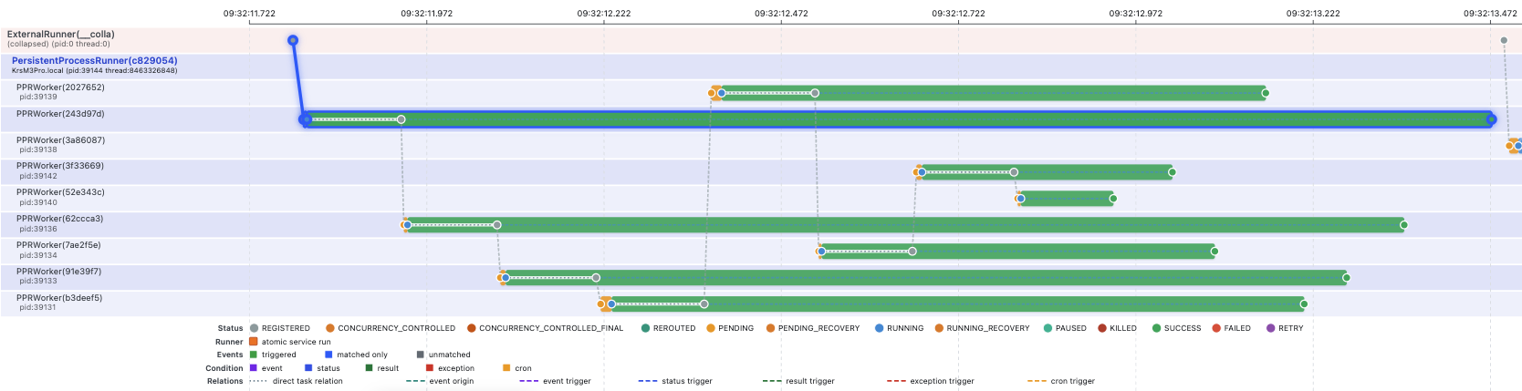
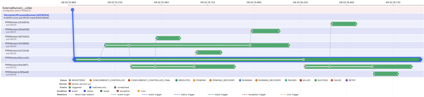
3. Breadth-first search: horizontal waves
For graph search, the sample uses this tree:
             A
          /  |  \
         B   C   D
        / \ / \ / \
       E  F G  H I  J
      / \
     K   L
BFS checks every node at the current depth before moving deeper. That is what produces the first wide task graph in the article.
The frontier is kept by a coordinator task. The node checks themselves are parallel task invocations:
@app.task
def inspect_breadth_first_node(
    graph: dict[str, list[str]],
    node: str,
    target: str,
    path: list[str],
) -> dict:
    time.sleep(STEP_DELAY_SECONDS)
    return {
        "path": path,
        "matched": node == target,
        "children": graph.get(node, []),
    }


@app.task
def breadth_first_search(graph, start, target):
    frontier = [[start]]
    visited = {start}

    while frontier:
        inspections = inspect_breadth_first_node.parallelize(
            {
                "graph": graph,
                "node": path[-1],
                "target": target,
                "path": path,
            }
            for path in frontier
        )
        level_results = list(inspections.results)
        # Return a match, or build the next frontier.
Searching from A to H produces three waves: A, then B C D, then the
nodes below them. BFS returns A -> C -> H, a shortest path in an unweighted
graph.
Unlike the list searches, several nodes from the same level can be inspected at the same time. A barrier is still imposed between levels: depth two cannot be assembled until the depth-one inspections return their children.
That matters for this demo. BFS can look much faster here because a whole frontier can be run across several workers at once. If only one worker were used, most of that advantage would disappear. The same nodes would still be visited, just not side by side.
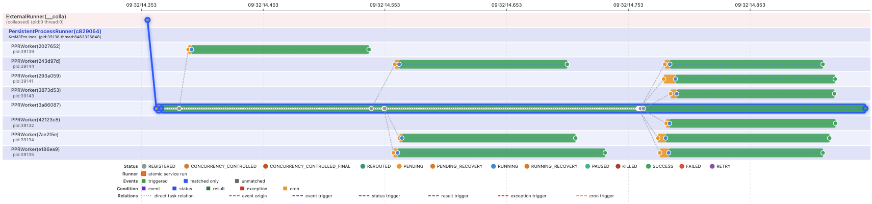
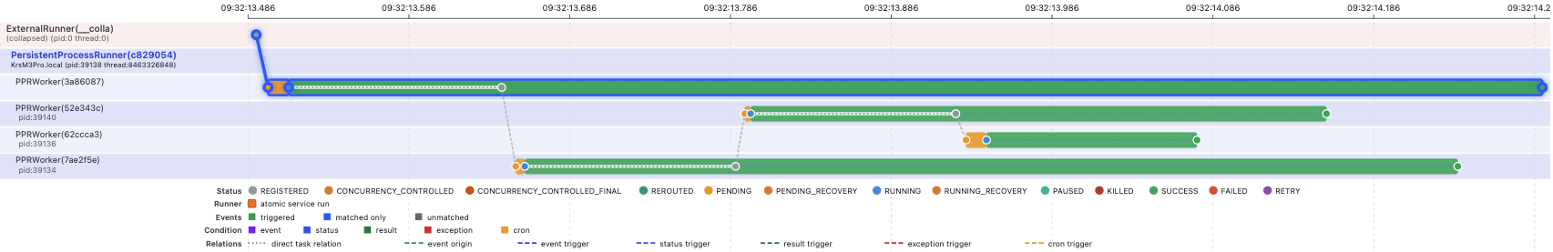
4. Depth-first search: one branch at a time
DFS uses the same graph and target, but follows one branch as far as it can before trying the next:
@app.task
def depth_first_search(
    graph: dict[str, list[str]],
    node: str,
    target: str,
    path: list[str] | None = None,
    visited: list[str] | None = None,
) -> list[str] | None:
    current_path = [*(path or []), node]
    current_visited = [*(visited or []), node]
    time.sleep(STEP_DELAY_SECONDS)

    if node == target:
        return current_path

    for child in graph.get(node, []):
        if child in current_visited:
            continue
        result = depth_first_search(
            graph, child, target, current_path, current_visited
        ).result
        if result is not None:
            return result
    return None
With the graph’s left-to-right ordering, DFS explores much of B’s subtree
before it reaches C and finds H. The final path is still A -> C -> H, but
the work leading to that answer is different.
The family tree should show nested invocations and backtracking rather than BFS’s wide levels. Both algorithms visit graph nodes. The interesting part here is how different the task graph looks.
The comparison
| Algorithm | Task graph | Useful parallelism here | Main visual |
|---|---|---|---|
| Linear search | One recursive chain | No | Long staircase |
| Binary search | One recursive chain | No | Short staircase |
| Breadth-first search | Coordinator plus parallel frontiers | Within each level | Horizontal waves |
| Depth-first search | Nested recursive branches | No in this implementation | Descent and backtracking |
The distributed version makes dependencies explicit, but the algorithms are not improved by default. Granularity matters. A task should normally contain enough work to justify routing, serialization, durable state, and coordination. A single integer comparison does not justify a broker.
That mismatch is the whole point of the demo. Pynmon can show:
- which invocation called which child
- which worker process ran each step
- how long parents waited for child results
- where BFS fan-out happened
- how DFS backtracking differs from level-order expansion
Run it
The quick path starts the runner, executes all four searches, and stops:
git clone https://github.com/pynenc/samples
cd samples/search_algorithms_demo
uv sync
uv run python sample.py
For visualizing, just run pynenc monitoring after the tests
uv run pynenc monitor
Open http://127.0.0.1:8000, then compare the invocation timeline and family trees. Keep the same zoom level when capturing linear versus binary, and BFS versus DFS; otherwise the comparison gets noisy.
What this does not prove
This demo does not benchmark search algorithms, Pynenc throughput, SQLite throughput, or process-pool sizing. The 120 ms sleeps dominate the runtime, the inputs are tiny, and the worker pool is intentionally oversubscribed.
A smaller point is being made instead: familiar algorithms have recognizable execution shapes, and durable task monitoring lets those shapes be inspected without everything being compressed into one Python stack trace.
That is enough for part one. Sorting algorithms should produce a different kind of mess.
Sample: https://github.com/pynenc/samples/tree/main/search_algorithms_demo.